Time series and nonlinear effects: Simulation-Inference
Haakon Bakka
BTopic 117 updated 2. December 2017
1 About
This is the Simulation-Inference counterpart to the Unemployment data example.
In this example we study when a complex model is identifiable, and how fast INLA will run.
1.1 Packages
library(INLA)
inla.setOption("num.threads", 1)
# - to only run 1 processor thread (no paralellisation)
set.seed(2017)
2 Simulation
2.1 Motivation
We have a long time series, for example temperature or unemployment. This time series contain no linear trends, as those would go to \(\pm \infty\).
We assume there is one seasonal effect, repeating every 12 months.
We assume there is one other covariate with a nonlinear effect.
2.2 Input parameters
We want to change these to try different things.
N = 3600
# - the number of observations
# - should be a multiple of 12
sig.epsilon = 0.5
# - the Gaussian noise
sig.u = 1
# - the structured part of the time series
rho = 0.90
# - the true autocorrelation
sig.seasonal = 2
# - the size of the seasonal effect
2.3 Simulation code
u = arima.sim(list(order = c(1,0,0), ar = rho), n = N,sd=1)
# - this sd is not the marginal standard deviation
u = u/sd(u)*sig.u
# - this has the correct standard deviation
seas.coeff = (0:11)*(1:12-12)
seas = rep(seas.coeff, N/12)
seas = drop(scale(seas))*sig.seasonalgaussian.error = rnorm(N, 0, sd=sig.epsilon)y = u + seas + gaussian.error3 Data
df = data.frame(y = y, t = 1:N, year = rep(1:12, N/12))plot(df$t, df$y, main="Data", col="blue")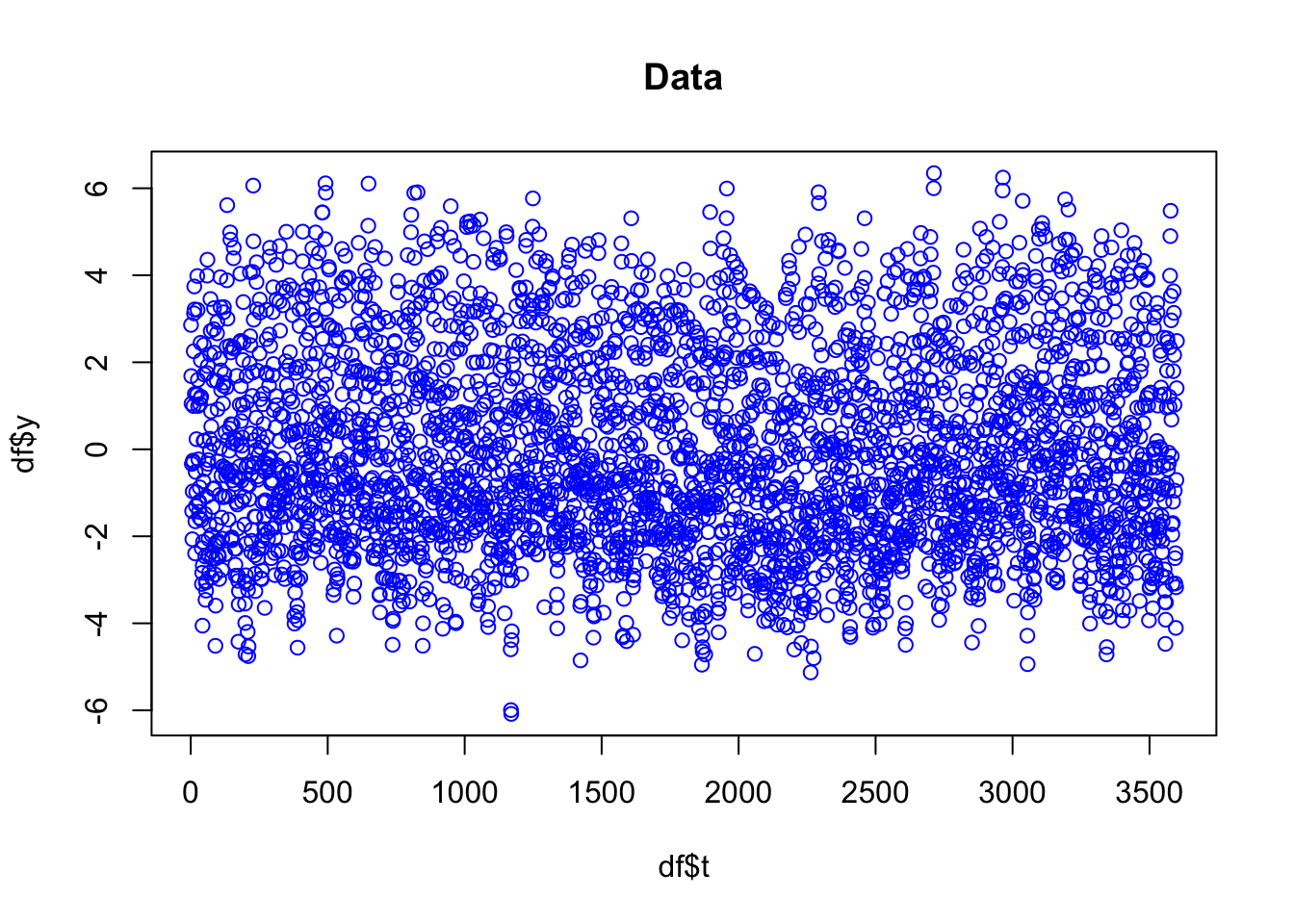
4 Model
hyper.ar1 = list(theta1 = list(prior="pc.prec", param=c(0.1, 0.5)),
                 theta2 = list(prior="pc.cor1", param=c(0.9, 0.5)))
hyper.rw2 = list(theta1 = list(prior="pc.prec", param=c(0.1, 0.5)))
hyper.family = list(theta = list(prior="pc.prec", param=c(3, 0.5)))
formula <- y~ f(t,model='ar1', hyper=hyper.ar1) + f(year, model="rw2", hyper=hyper.rw2, cyclic=T, constr=T)
res <- inla(formula=formula, data=df, family="gaussian",
control.predictor=list(compute=TRUE),
control.family = list(hyper = hyper.family))5 Result
summary(res)##
## Call:
## c("inla.core(formula = formula, family = family, contrasts =
## contrasts, ", " data = data, quantiles = quantiles, E = E,
## offset = offset, ", " scale = scale, weights = weights,
## Ntrials = Ntrials, strata = strata, ", " lp.scale = lp.scale,
## link.covariates = link.covariates, verbose = verbose, ", "
## lincomb = lincomb, selection = selection, control.compute =
## control.compute, ", " control.predictor = control.predictor,
## control.family = control.family, ", " control.inla =
## control.inla, control.fixed = control.fixed, ", " control.mode
## = control.mode, control.expert = control.expert, ", "
## control.hazard = control.hazard, control.lincomb =
## control.lincomb, ", " control.update = control.update,
## control.lp.scale = control.lp.scale, ", " control.pardiso =
## control.pardiso, only.hyperparam = only.hyperparam, ", "
## inla.call = inla.call, inla.arg = inla.arg, num.threads =
## num.threads, ", " blas.num.threads = blas.num.threads, keep =
## keep, working.directory = working.directory, ", " silent =
## silent, inla.mode = inla.mode, safe = FALSE, debug = debug, ",
## " .parent.frame = .parent.frame)")
## Time used:
## Pre = 3.19, Running = 3.71, Post = 0.0839, Total = 6.99
## Fixed effects:
## mean sd 0.025quant 0.5quant 0.97quant mode kld
## (Intercept) -0.046 0.07 -0.18 -0.046 0.086 -0.046 0
##
## Random effects:
## Name Model
## t AR1 model
## year RW2 model
##
## Model hyperparameters:
## mean sd 0.025quant
## Precision for the Gaussian observations 4.126 0.212 3.725
## Precision for t 0.987 0.070 0.854
## Rho for t 0.890 0.010 0.871
## Precision for year 1.848 0.627 0.883
## 0.5quant 0.97quant mode
## Precision for the Gaussian observations 4.120 4.543 4.107
## Precision for t 0.985 1.123 0.984
## Rho for t 0.891 0.908 0.891
## Precision for year 1.761 3.241 1.596
##
## Marginal log-Likelihood: -4139.73
## is computed
## Posterior summaries for the linear predictor and the fitted values are computed
## (Posterior marginals needs also 'control.compute=list(return.marginals.predictor=TRUE)')plot(df$y, res$summary.fitted.values$mean, main="Fitting result")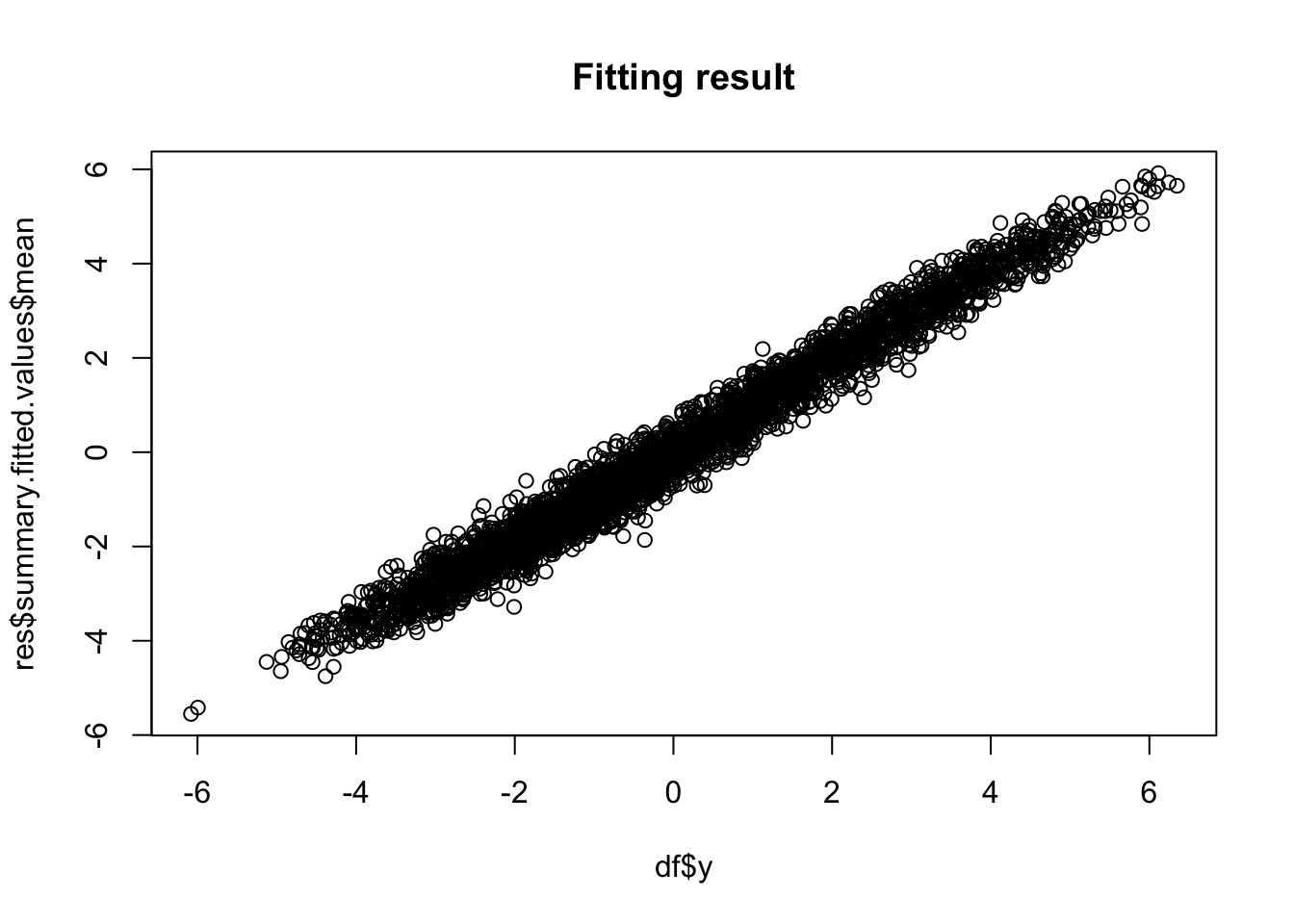
6 Estimation of the hyper-parameters
Here we plot prior, posterior and truth!
Figuring out how to plot these is not trivial, and will take some time. However, it is not a good topic to talk about in detail during a course.
6.1 \(\sigma_\epsilon\)
marginal = res$internal.marginals.hyperpar$`Log precision for the Gaussian observations`
transform = function(x) exp(-0.5*x)
sig.eps.posterior = inla.tmarginal(transform, marginal)

plot(sig.eps.posterior, type="l", xlab = expression(sigma), ylab = "Probability density",
     main = "Size of noise component")

xvals = seq(0.45, 0.62, length.out=1000)
lambda = -log(hyper.family$theta$param[2])/hyper.family$theta$param[1]
lines(xvals, 1E1*exp(-lambda*xvals), lty='dashed')
abline(v=sig.epsilon, col="blue")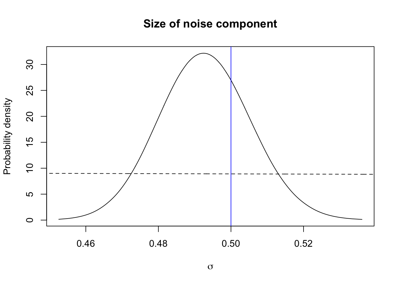
The blue vertical line is the true value, the dashed line is the prior, and the full line is the posterior.
6.2 \(\sigma_\epsilon\)
marginal = res$internal.marginals.hyperpar$`Log precision for t`
transform = function(x) exp(-0.5*x)
sig.posterior = inla.tmarginal(transform, marginal)

plot(sig.posterior, type="l", xlab = expression(sigma), ylab = "Probability density",
     main = "Size of AR1 component")

xvals = seq(0.5, 1.5, length.out=1000)
lambda = -log(hyper.ar1$theta1$param[2])/hyper.ar1$theta1$param[1]
lines(xvals, 1E3*exp(-lambda*xvals), lty='dashed')
abline(v=sig.u, col="blue")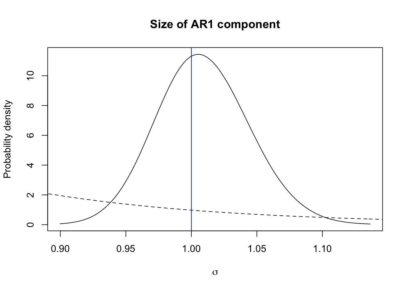
The blue vertical line is the true value, the dashed line is the prior, and the full line is the posterior.
6.3 \(\rho\)
Here we can use the standard output marginal in INLA.
marginal = res$marginals.hyperpar$`Rho for t`

plot(marginal, type="l", xlab = expression(sigma), ylab = "Probability density",
     main = "Correlation of AR1 component", xlim=c(0.87, 1))

xvals = seq(0.85, 1, length.out=1000)
lines(xvals, 5*inla.pc.dcor1(xvals, hyper.ar1$theta2$param[1],
                              hyper.ar1$theta1$param[2]), lty='dashed')

abline(v=rho, col="blue")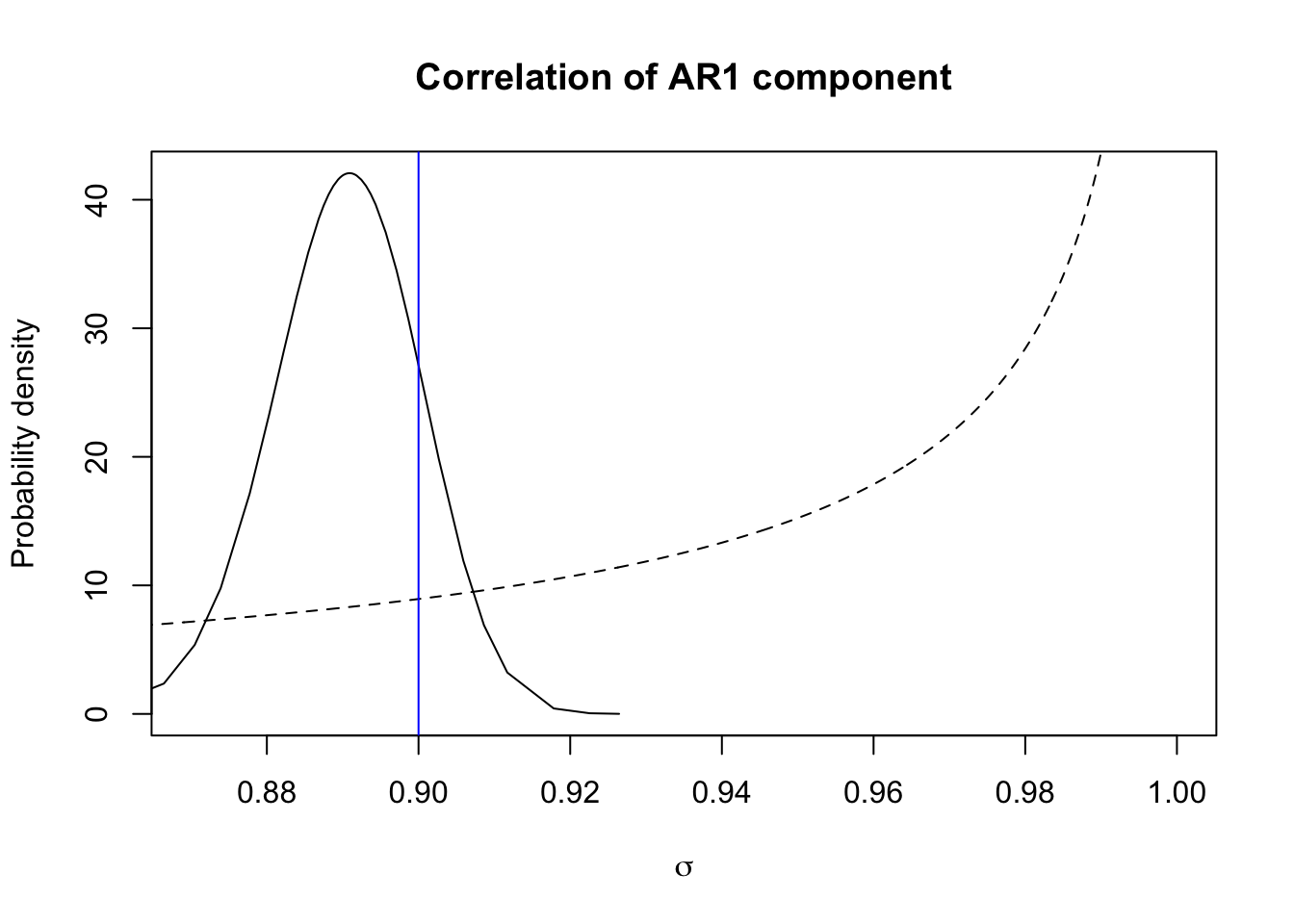
The blue vertical line is the true value, the dashed line is the prior, and the full line is the posterior.
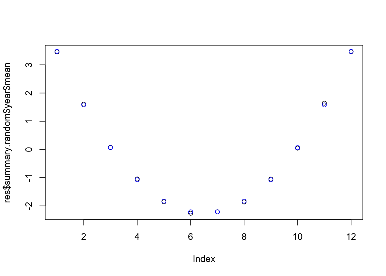
6.4 The seasonal effect
plot(res$summary.random$year$mean)
points(seas, col="blue")