1 About

1.1 Packages
1.2 Model component 1: AR1
1.3 The precision matrix

2 Calculate $Q$ entries

2.1 An important detail we will skip
2.2 Create a function

3 Use sparse matrices

3.1 Note for implementation

4 Compute probabilities with $Q$

4.1 Cholesky
4.2 Computing determinant of $Q$
4.3 Computing a probability

5 Sample from $\mathcal N(0, Q)$

1 About

In this topic we compute with the precision matrix for the AR1 model component.

Calculate $Q$ entries
Use sparse matrices (not keep the 0s)
Compute probabilities with $Q$
Sample from $\mathcal N(0, Q)$

1.1 Packages

library(INLA)

1.2 Model component 1: AR1

We model $u$ as an autoregressive model of order 1 over time t.

This is described as $u_t = \rho u_{t-1} + \epsilon_t$ where $\epsilon_t$ is iid Gaussian randomness.

The two hyper-parameters for this component are $\rho$ and the marginal standard deviation $\sigma_u$ .

1.3 The precision matrix

The this topic is about is the $Q$ matrix in ${u} \sim \mathcal N(0, Q^ {-1})$

2 Calculate $Q$ entries

Per definition of precision matrix $\log(\pi(u)) = c - \frac{1}{2} u^\top Q u.$

Rewrite definition of our model component as a function of $\epsilon$ . $\epsilon_t = u_t - \rho u_{t-1},$ giving the joint distribution $\log(\pi(u)) = c - \frac{1}{2} (\epsilon_2^2 + \epsilon_3^2 + \epsilon_4^2 + ... + \epsilon_T^2) .$ Further, $\log(\pi(u)) = c - \frac{1}{2} ((u_2 - \rho u_{1})^2 + (u_3 - \rho u_{2})^2 + (u_4 - \rho u_{3})^2 + ... + (u_T - \rho u_{T-1})^2) .$

Matching this term to the $Q$ matrix, we get $u^\top Q u = u_2^2 -2 \rho u_2 u_1 + \rho^2u_1^2 + u_3^2 -2\rho u_3u_2 + \rho^2u_2 + u_4^2 -2\rho u_4u_3 + \rho^2u_3 +...$

By experimenting a bit with the $u^\top Q u$ (quadratic) form, we see that the only way to make a symmetric $Q$ is by definig the following $Q$ .

N = 10
rho = 0.95
Q = matrix(0, N, N)
diag(Q) = 1+rho^2
for (i in 1:(N-1)) {
  Q[i, i+1] = -rho
  Q[i+1, i] = -rho
}
print(Q)

##        [,1]  [,2]  [,3]  [,4]  [,5]  [,6]  [,7]  [,8]  [,9] [,10]
##  [1,]  1.90 -0.95  0.00  0.00  0.00  0.00  0.00  0.00  0.00  0.00
##  [2,] -0.95  1.90 -0.95  0.00  0.00  0.00  0.00  0.00  0.00  0.00
##  [3,]  0.00 -0.95  1.90 -0.95  0.00  0.00  0.00  0.00  0.00  0.00
##  [4,]  0.00  0.00 -0.95  1.90 -0.95  0.00  0.00  0.00  0.00  0.00
##  [5,]  0.00  0.00  0.00 -0.95  1.90 -0.95  0.00  0.00  0.00  0.00
##  [6,]  0.00  0.00  0.00  0.00 -0.95  1.90 -0.95  0.00  0.00  0.00
##  [7,]  0.00  0.00  0.00  0.00  0.00 -0.95  1.90 -0.95  0.00  0.00
##  [8,]  0.00  0.00  0.00  0.00  0.00  0.00 -0.95  1.90 -0.95  0.00
##  [9,]  0.00  0.00  0.00  0.00  0.00  0.00  0.00 -0.95  1.90 -0.95
## [10,]  0.00  0.00  0.00  0.00  0.00  0.00  0.00  0.00 -0.95  1.90

2.1 An important detail we will skip

A confusing part of the AR1 model is that we must define the first value to have the correct distribution to make the process stationary, see inla.doc("ar1") for details. We fix this now:

Q[1,1] = 1
Q[N,N] = 1

2.2 Create a function

For comparison later, we now create a function for $Q$ , summarising our computations so far.

precision.ar1 = function(N, rho){
  Q = matrix(0, N, N)
  diag(Q) = 1+rho^2
  for (i in 1:(N-1)) {
    Q[i, i+1] = -rho
    Q[i+1, i] = -rho
  }
  Q[1,1] = 1
  Q[N,N] = 1
  return(Q)
}

3 Use sparse matrices

The matrix $Q$ we have created stores all the zeroes! Let us convert this to a sparse matrix and compare them.

Q = precision.ar1(10, 0.9)
print(Q)

##       [,1] [,2] [,3] [,4] [,5] [,6] [,7] [,8] [,9] [,10]
##  [1,]  1.0 -0.9  0.0  0.0  0.0  0.0  0.0  0.0  0.0   0.0
##  [2,] -0.9  1.8 -0.9  0.0  0.0  0.0  0.0  0.0  0.0   0.0
##  [3,]  0.0 -0.9  1.8 -0.9  0.0  0.0  0.0  0.0  0.0   0.0
##  [4,]  0.0  0.0 -0.9  1.8 -0.9  0.0  0.0  0.0  0.0   0.0
##  [5,]  0.0  0.0  0.0 -0.9  1.8 -0.9  0.0  0.0  0.0   0.0
##  [6,]  0.0  0.0  0.0  0.0 -0.9  1.8 -0.9  0.0  0.0   0.0
##  [7,]  0.0  0.0  0.0  0.0  0.0 -0.9  1.8 -0.9  0.0   0.0
##  [8,]  0.0  0.0  0.0  0.0  0.0  0.0 -0.9  1.8 -0.9   0.0
##  [9,]  0.0  0.0  0.0  0.0  0.0  0.0  0.0 -0.9  1.8  -0.9
## [10,]  0.0  0.0  0.0  0.0  0.0  0.0  0.0  0.0 -0.9   1.0

Q = precision.ar1(10, 0.9)
Q = as(Q, "sparseMatrix")
print(Q)

## 10 x 10 sparse Matrix of class "dsCMatrix"
##                                                        
##  [1,]  1.0 -0.9  .    .    .    .    .    .    .    .  
##  [2,] -0.9  1.8 -0.9  .    .    .    .    .    .    .  
##  [3,]  .   -0.9  1.8 -0.9  .    .    .    .    .    .  
##  [4,]  .    .   -0.9  1.8 -0.9  .    .    .    .    .  
##  [5,]  .    .    .   -0.9  1.8 -0.9  .    .    .    .  
##  [6,]  .    .    .    .   -0.9  1.8 -0.9  .    .    .  
##  [7,]  .    .    .    .    .   -0.9  1.8 -0.9  .    .  
##  [8,]  .    .    .    .    .    .   -0.9  1.8 -0.9  .  
##  [9,]  .    .    .    .    .    .    .   -0.9  1.8 -0.9
## [10,]  .    .    .    .    .    .    .    .   -0.9  1.0

The “.” signifies that the zeroes are not stored. How is this done instead? A list of indices $(i,j)$ together with their value $x_{i,j}$ are stored as 3 lists.

str(Q)

## Formal class 'dsCMatrix' [package "Matrix"] with 7 slots
##   ..@ i       : int [1:19] 0 0 1 1 2 2 3 3 4 4 ...
##   ..@ p       : int [1:11] 0 1 3 5 7 9 11 13 15 17 ...
##   ..@ Dim     : int [1:2] 10 10
##   ..@ Dimnames:List of 2
##   .. ..$ : NULL
##   .. ..$ : NULL
##   ..@ x       : num [1:19] 1 -0.9 1.81 -0.9 1.81 -0.9 1.81 -0.9 1.81 -0.9 ...
##   ..@ uplo    : chr "U"
##   ..@ factors : list()

As you see, this “dgCMatrix” uses $p$ instead of $j$ , storing the entries in a slightly different way.

What is all the fuzz about?

for (N in c(10, 1E2, 1E3, 5E3 )) {
  Q = precision.ar1(N, 0.9)
  os1 = round(object.size(Q)/1000)
  Q = as(Q, "sparseMatrix")
  os2 = round(object.size(Q)/1000)
  print(paste0("For N is ", N, " we go from ", os1, " kb to ", os2, " kb"))
}

## [1] "For N is 10 we go from 1 kb to 2 kb"
## [1] "For N is 100 we go from 80 kb to 5 kb"
## [1] "For N is 1000 we go from 8000 kb to 30 kb"
## [1] "For N is 5000 we go from 2e+05 kb to 142 kb"

3.1 Note for implementation

Creating a full matrix and then using as.sparse is bad practice. You should create the i, j, x indices/values and use ?sparseMatrix. Your entire inference algorithm, for large problems, might be quicker than writing down the full matrix even once.

4 Compute probabilities with $Q$

4.1 Cholesky

The basic part of computing with precision matrices is being able to do the cholesky factorisation to get $Q = L L^\top$ .

Q = precision.ar1(1000, 0.99)
L = chol(Q)
print(sum(abs(Q- t(L)%*%L)))

## [1] 0

4.2 Computing determinant of $Q$

We know that $det(Q) = det(L^ \top) det(L) = det(L)^ 2.$ It is very important to know that we never want to compute determinants, only log-determinants. Similarly to how we never compute probabilities only log probabilities. This is because of numerical stability (if you don’t take the log, most things are infinite or zero).

$logdet(Q) = 2 logdet(L)$ How to find the determinant of $L$ ? Since the cholesky is lower or upper triangular, we can just take the product of the diagonal! If you look at the matrix $L$ this is actually upper triangular, since this is R default.

$logdet(Q) = 2 \sum_i \log(L_{i,i})$

4.3 Computing a probability

Assume that we want to compute the (joint) probability that $u_i=0.1$ for all $i$ simultaneously (as an example).

The general formula $\log(\pi(u)) = \frac{1}{2}\log \left| (2\pi)^ {-1} Q \right| - \frac{1}{2} \vec u^\top Q \vec u$ gives us $\log(\pi(u=0.1)) = -\frac{N}{2}\log(2\pi) + \frac{1}{2}\log \left| Q \right| - \frac{1}{2} 0.1^\top Q 0.1.$

In code this is:

pt1 = rep(0.1, nrow(Q))
log.prob.pt1 = -nrow(Q)/2*log(2*pi) + 0.5*2*sum(log(diag(L))) - 0.5 *pt1 %*% Q %*% pt1
print(log.prob.pt1)

##      [,1]
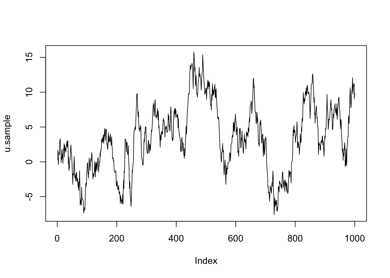
## [1,] -921

5 Sample from $\mathcal N(0, Q)$

To sample from $Q$ we just define $u$ as the solution to $Lu = z$ where $z$ are iid Gaussians $\mathcal N(0, 1)$ . Then $precision(u) = L^\top L.$ The sampling code we can write as follows.

set.seed(2017)
z.sample = rnorm(nrow(Q))
u.sample = solve(L, z.sample)
plot(u.sample, type="l")

Basic computations with precision matrix: AR1 example

Haakon Bakka

BTopic120 updated 10. March 2017

1 About

1.1 Packages

1.2 Model component 1: AR1

1.3 The precision matrix

2 Calculate $Q$ entries

2.1 An important detail we will skip

2.2 Create a function

3 Use sparse matrices

3.1 Note for implementation

4 Compute probabilities with $Q$

4.1 Cholesky

4.2 Computing determinant of $Q$

4.3 Computing a probability

5 Sample from $\mathcal N(0, Q)$

Basic computations with precision matrix: AR1 example

Haakon Bakka

BTopic120 updated 10. March 2017

1 About

1.1 Packages

1.2 Model component 1: AR1

1.3 The precision matrix

2 Calculate QQ entries

2.1 An important detail we will skip

2.2 Create a function

3 Use sparse matrices

3.1 Note for implementation

4 Compute probabilities with QQ

4.1 Cholesky

4.2 Computing determinant of QQ

4.3 Computing a probability

5 Sample from N(0,Q)\mathcal N(0, Q)

2 Calculate $Q$ entries

4 Compute probabilities with $Q$

4.2 Computing determinant of $Q$

5 Sample from $\mathcal N(0, Q)$