Polygons and Coastlines
Francesco Serafini
Runbing Zheng
Haakon Bakka
updated 16 March 2021
1 About
In this page we explain how to build polygons with the
INLA and sp packages. This functionality is
very useful in particular when we are dealing with physical barriers,
which are important in statistical models on maps (spatial statistics).
On this page we show several practical examples of how to deal with
polygons. After that we show how to create polygons representing a
geographical area of interest, how to build a mesh on this area, and how
to get some nice plot from Google Maps.
1.1 Polygons for Physical Boundaries
In many real spatial models we have to deal with areas with physical boundaries. Let us think about data coming from sensors placed in the sea recording a signal which doesn’t propagate on the earth. In this situation any island represents a physical boundary that we have to take into account when modeling. On the other hand we could think of the opposite situation: We are interested in what happens on land and do not care about the sea, and the sea acts as a boundary, e.g. in disease mapping. For these boundaries, Haakon developed the Barrier model, see Btopic128. This topic is also a guidance on how to make meshes for the Barrier model.
1.2 Polygons in general for mesh construction
More in general, having a mesh with holes is useful in some situations. Let us think about the following scenario: we have an area in which the data is missing. We can’t simply ignore that part of the total area. One possible solution is to treat it as an hole and then build a mesh with larger triangles on the missing data area. Then we get a continuous process over all of space, but we have less mesh nodes in the holes, and therefore faster computations.
1.3 Libraries
library(INLA)
library(rgdal)
library(rgeos)
library(ggmap)
set.seed(2018)
2 Simple constructed polygons
First, we show an example of simple polygons that we construct manually. Our real polygon example is not dependent on this simple example. However, if you want to study the R objects, and how they behave, it is better to start with this simple example.
2.1 Basic Polygon
Let us create a simple study area composed of two parts. The first
one has a hole and the second is non-convex. We can do that using the
\(\texttt{Polygons()}\) function of the
sp package, which creates an object of class Polygons. This
function needs just two arguments:
coords: 2 column numeric matrix with the coordinates of the vertices of the polygon.hole: logical value for setting polygon as hole or not.
Let us define our first polygon. Similar code can be found in the SPDE-book.
# First polygon
pl1 <- Polygon(cbind(c(0,15,15,0,0), c(5,0,20,20,5)), hole=FALSE)
# Hole in the first polygon
h1 <- Polygon(cbind(c(5,12,10,5,5), c(7,7,15,15,7)), hole=TRUE)
# Second polygon
pl2 <- Polygon(cbind(c(15,20,20,30,30,15,15), c(10,10,0,0,20,20,10)), hole=FALSE)
The function \(\texttt{SpatialPolygons()}\) is used to
create a single object containing the two above polygons. The function
takes as argument a list of lists and gives as output an object of class
SpatialPolygons.
sp <- SpatialPolygons(list(Polygons(list(pl1, h1), '0'),
                           Polygons(list(pl2), '1')))
plot(sp, main = 'Polygon')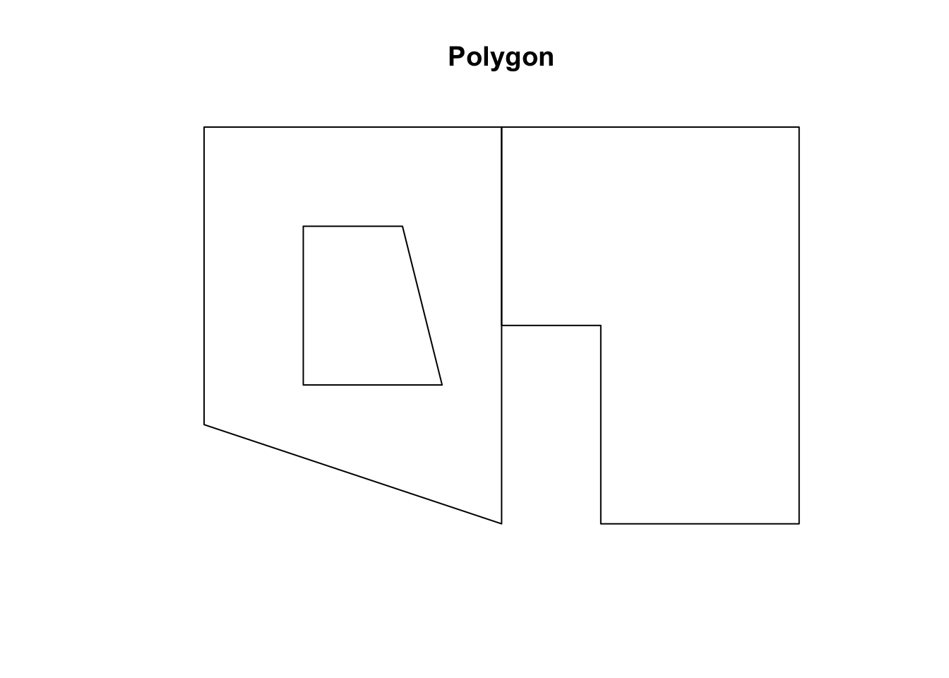
2.2 Mesh construction on this polygon
mesh <- inla.mesh.2d(boundary=sp, max.edge=2)
plot(mesh, main = 'Mesh')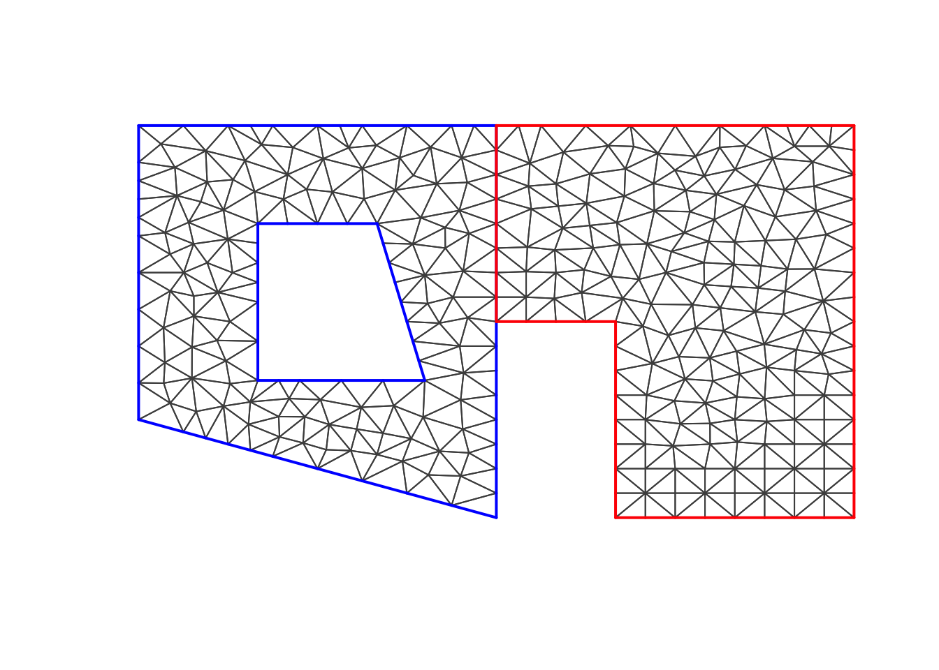
One could be interested in building a finer mesh on the areas of interest and a poorer one in the other regions (the holes) of the study area. It is possible to do that just expanding the study area.
mesh2 <- inla.mesh.2d(boundary=sp, max.edge=c(1,4))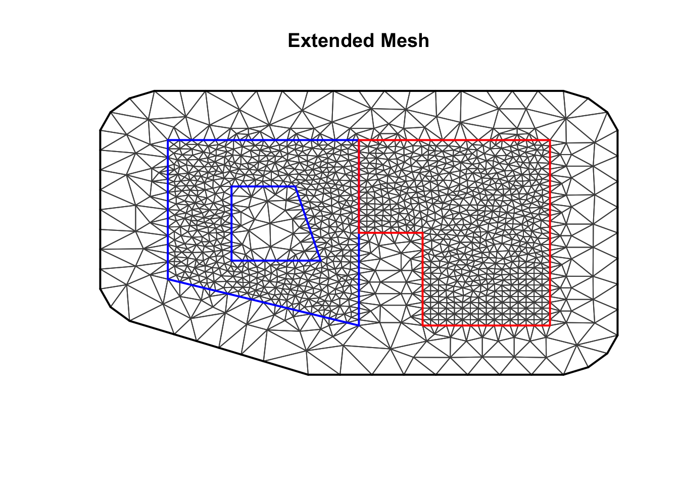
3 Polygons from coastlines
As we said before in many applications in geographical statistics it is necessary to deal with coastlines. In this section we show how to use real world coastlines data in order to create a polygon for our study area.
3.1 Download Coastlines Data
First of all we need to downlad the shape file of the coastlines. The data is available on this webpage:
http://openstreetmapdata.com/data/coast
We will take “Large simplified polygons not split, use for zoom level
0-9” as an example, to show how to get region polygons from this
dataset. We import the data using rgdal library:
Notice that the dsn need to point to the file directory
with the downloaded files.
We try to make all the code in this tutorial with
eval=TRUE, so that you can run it. However, the next few
code chunks are with eval=FALSE, and you cannot simply run
them. This is because we cannot make the world shapefile accessible from
this website (you have to go to http://openstreetmapdata.com/data/coast). After you have
downloaded the correct data, you can manually run the code chunks (note
that they are somewhat time consuming). Further down on this page we go
back to eval=TRUE.
shape <- readOGR(dsn = ".", layer = "simplified_land_polygons")## OGR data source with driver: ESRI Shapefile
## Source: ".", layer: "simplified_land_polygons"
## with 63019 features
## It has 1 fields
## Integer64 fields read as strings: FIDWe cannot plot shape using directly the \(\texttt{ plot()}\) function because it
requires a lot of time to render. Have in mind that we are talking about
more than sixty thousands polygons! One way to render a nice plot is to
save it directly as a png; this little trick almost always works.
png("fig/btopic127/shapeplot1.png", width = 480*4, height=480*4)
plot(shape)
dev.off()

# Open the saved file to see the following plot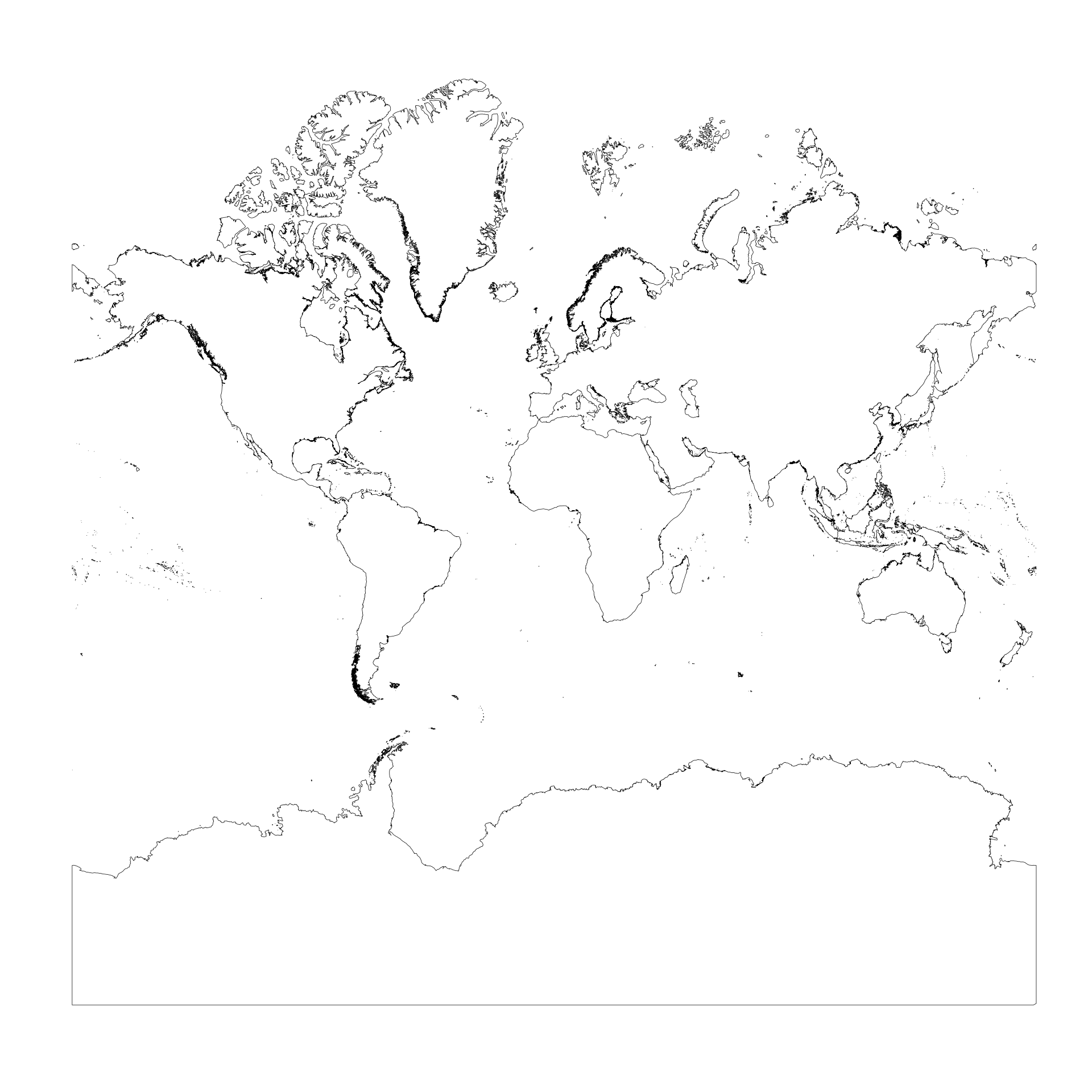
3.2 Transform the shapefile and select an area
Once we have the shapefile is useful to perform a latitude longitude projection. In this way we will be able to select the area of interested using the coordinates.
shape2 <- spTransform(shape, CRS("+proj=longlat +datum=WGS84"))Take a look, just to check whats going on
png("fig/btopic127/shapeplot2.png", width = 480*4, height=480*4)
plot(shape2)
dev.off()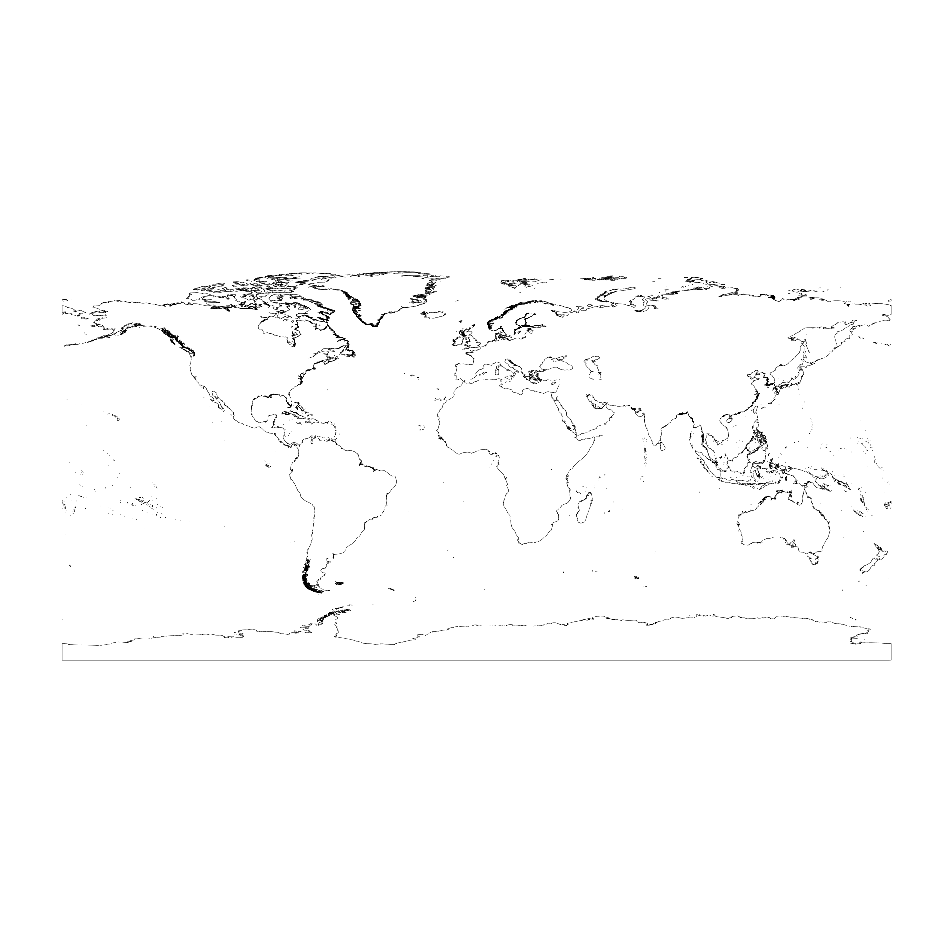
Now we can select the area of interest using the coordinates. Notice
that the longitude and latitude can be easily retrivied using Google
Maps (by clicking a point on the map and reading off the
coordinates).
As an example we select some islands in the south of Greece.
png("fig/btopic127/shapeplot3.png", width = 480*4, height=480*4)
plot(shape2, xlim=c(22.80, 26.85), ylim=c(34.88, 38.06))
dev.off()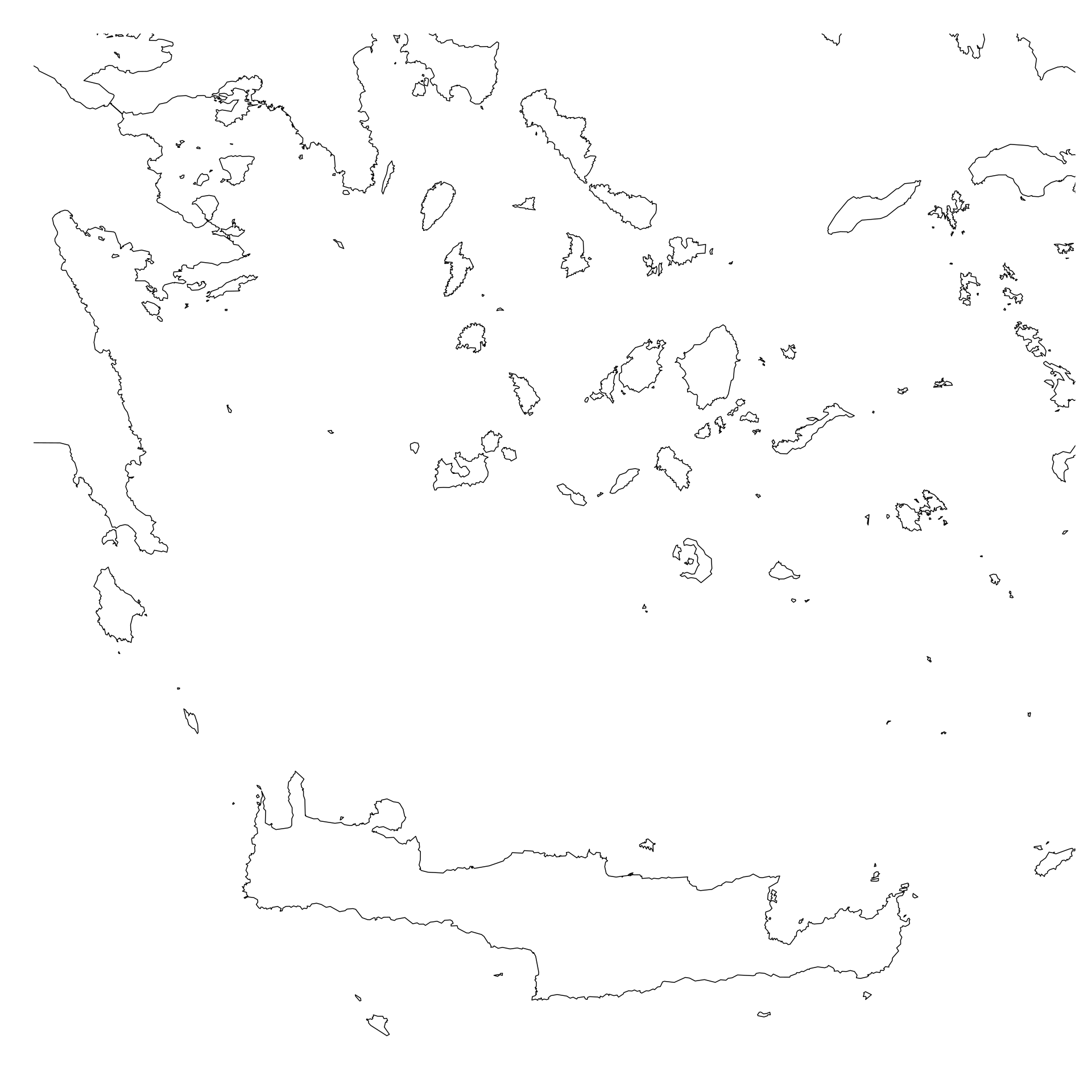
3.3 Creating Polygons
Now that we have an area of interest we can start building our polygons. The first thing we need is a polygon representing the study area. This will be our starting point (representing the sea) and then we will add holes (islands) to it.
# You can run this code chunk
pl1 <- Polygon(cbind(c(22.80, 22.80, 26.85, 26.85, 22.80),
                     c(38.06, 34.88, 34.88, 38.06, 38.06)), hole=FALSE)
sp <- SpatialPolygons(list(Polygons(list(pl1), '0')),
                      proj4string =CRS("+proj=longlat +datum=WGS84"))
The next step is to create polygons representing the islands; in the
end we will turn this polygons into holes. In order to create the
polygons, we need to intersect our square polygon with the shapefile.
Warning: This operation can take roughly half an hour to run. This gets
even worse if you are working with large areas. To intersect the polygon
with the shape file we used functions from the rgeos
library.
shape3 <- gBuffer(shape2, byid=TRUE, width=0) #for gIntersection operation
shape4 <- gIntersection(shape3, sp) #this is the heavy guy
shape5 = gSimplify(shape4, tol=0.001) #use tol to control the precision
Notice that:
For a large area,
shape4is Large SpatialPolygonsDataFrame and needs@polyobjto get the Spatial Polygons for the following operation.For a small area,
shape4is Formal class SpatialPolygons. So we can just use it.The function \(\texttt{gSimplify()}\) gives us a more regular and light shape file. Working with this file makes the mesh more regular and reduces the computational time (recommended for large area).
Now that we have a simplified version of our shapefile of interest we
can save it. In this way, in the future we can simply import it and work
directly on the area of interest. Note that to be saved the file should
be a SpatialPolygonsDataFrame. The following code will
create a folder call “temp” with the shape file inside.
shape_df = as(shape5, 'SpatialPolygonsDataFrame')
writeOGR(shape_df, layer = 'shape5','temp/' ,driver="ESRI Shapefile")
To import the shape file we can use the same command as before. From now on, until the end of the page, you can run the code (we use ‘eval=TRUE’). [add where to download the shape file TODO: Haakon]
shape5 <- readOGR(dsn = "data/btopic127/", layer = "shape5")## Warning: OGR support is provided by the sf and terra packages among
## others## Warning: OGR support is provided by the sf and terra packages among
## others## Warning: OGR support is provided by the sf and terra packages among
## others## Warning: OGR support is provided by the sf and terra packages among
## others## Warning: OGR support is provided by the sf and terra packages among
## others## Warning: OGR support is provided by the sf and terra packages among
## others## OGR data source with driver: ESRI Shapefile
## Source: "/Users/haakonbakka/Documents/GitHub/hc-private-code-and-web/web/webpage-source/data/btopic127", layer: "shape5"
## with 1 features
## It has 1 fieldsFinally, we are ready to build our mesh with holes.
# create a polygon representing the area of interest
pll = Polygon(sp@polygons[[1]]@Polygons[[1]]@coords, hole = F)

# number of polygons representing the islands
n_poly = length(shape5@polygons[[1]]@Polygons)
idx = seq(1:n_poly)

# create a list of holes
hole_list = lapply(idx, function(n) Polygon(shape5@polygons[[1]]@Polygons[[n]]@coords, hole = T))

# create the final Spatial Polygons
new_sp = SpatialPolygons(list(Polygons(append(hole_list, pll),'1')))

# take a look
plot(new_sp)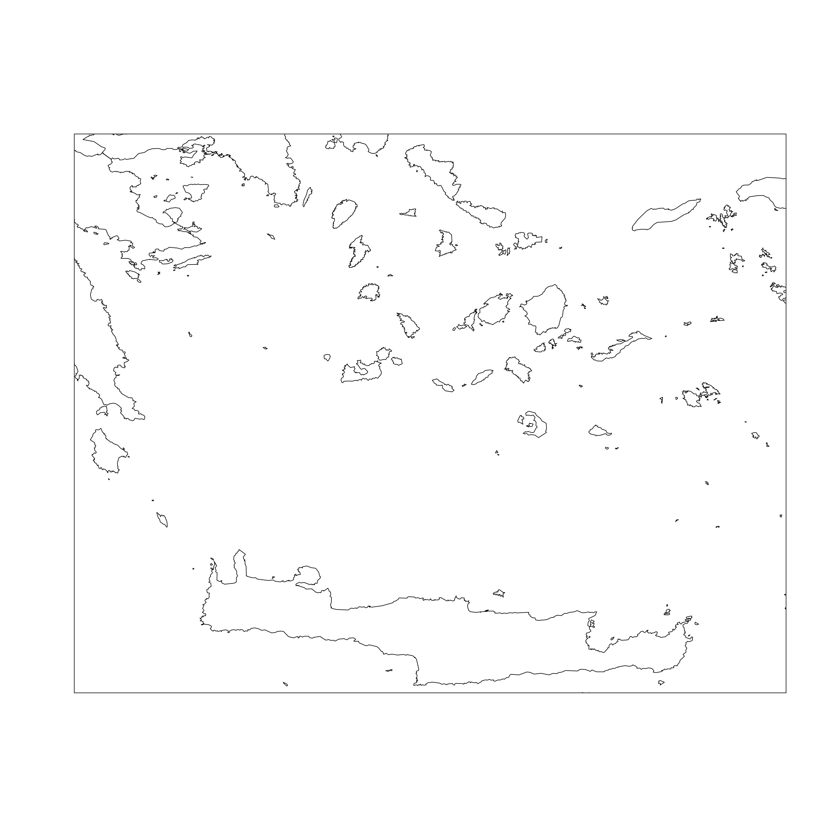
4 Build a mesh from this polygon
In this section we show how to build a mesh from the polygon we just made. A similar example can be found in BTopic104.
mesh_poly = inla.mesh.2d(boundary = new_sp, max.edge = 0.2)
plot(mesh_poly, main = '')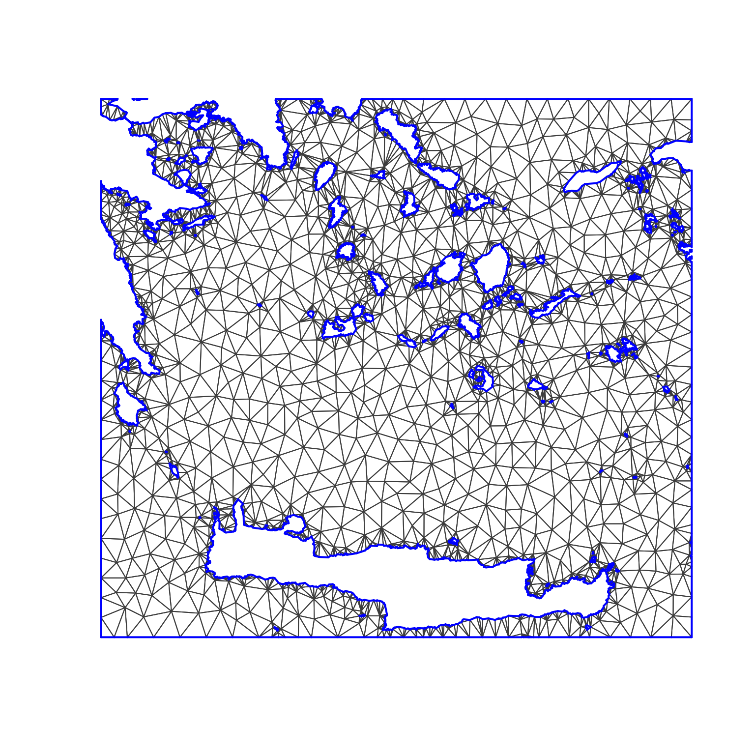
Lets extend the study area. See BTopic104 for how to specify the parameters to build a good mesh.
mesh_poly2 = inla.mesh.2d(boundary = new_sp, max.edge = c(0.1, 0.4),
                          cutoff = c(0.02))
plot(mesh_poly2, main = '')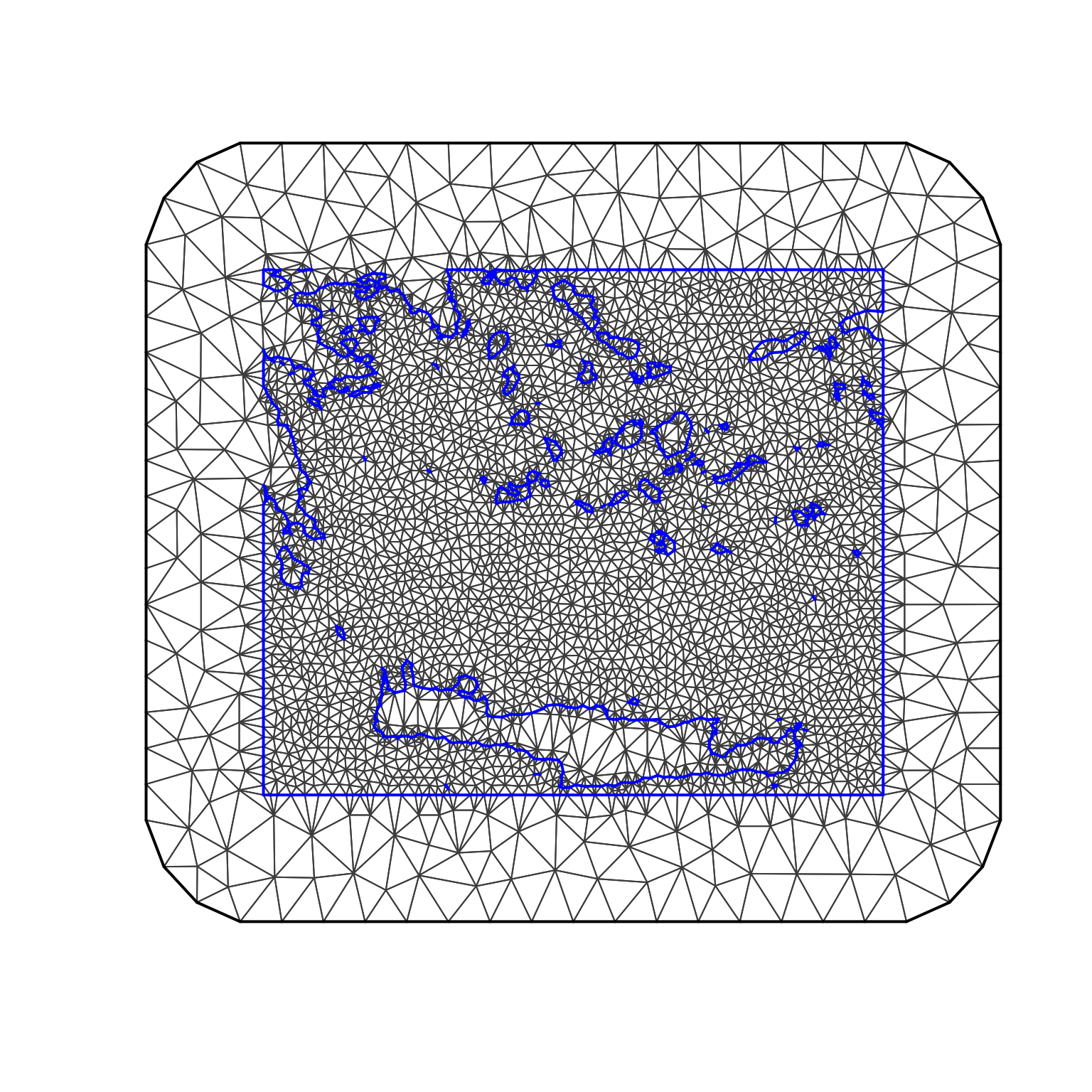
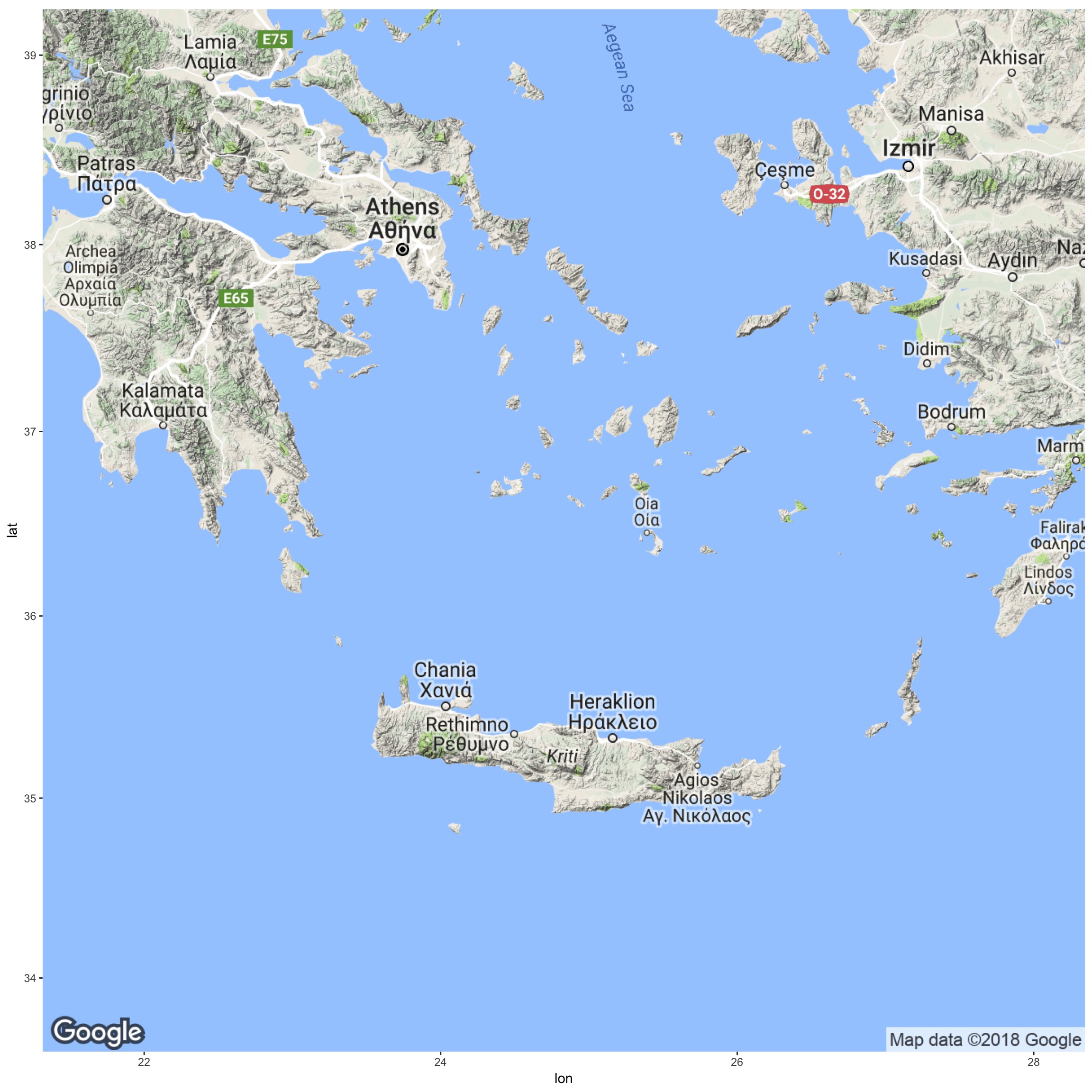
5 Plotting Maps
5.1 Map from Google
This last section is dedicated to how to use the shape file to have a
nice plot using the ggmap library. Let us import the map
from Google.
try({
  glgmap = get_map(location = shape5@bbox, maptype= "terrain", zoom = 7)
  p = ggmap(glgmap) #p is the plot of glgmap
  print(p)
})
## Error in get_googlemap(center = location, zoom = zoom, maptype = maptype, :
## Google now requires an API key; see
## `ggmap::register_google()`.In case you have problems compiling this, we insert the plot below
for comparison.
We now highlight the area of interest.
try({
  p1 = p + xlab("Longitude") + ylab("Latitude")
  p2 = p1 + geom_polygon(data = fortify(shape5),
                       aes(long, lat, group = group),
                       fill = "orange", colour = "red", alpha = 0.2)
  p3 = p2 + geom_polygon(data = fortify(sp),
                       aes(long, lat, group = group),
                       fill = NA, colour = "black", alpha = 1)
  print(p3)
})
## Error in p + xlab("Longitude") : non-numeric argument to binary operatorAgain, we manually insert the plot below.

5.2 Transform the Data to UTM
UTM is one of the most common map projections today. The most important attribute of UTM is that it represents the size/dimensions of the area accurately. Let us transform the shape file into this format. Note that longitude and latitude is not a good representation! The procedure is the same as before, and we use the same function used for latitude longitude projection.
#```{r, message = F, fig.width=8, fig.height=8}
## 13th april 2023:
## This code no longer runs! Bummer!
## If anyone knows how to fix, please let me know!
try({
  shape_utm = spTransform(shape5, CRS("+proj=utm +zone=35S ellps=WGS84"))
  plot(shape_utm)
})
## Error in h(simpleError(msg, call)) :
## error in evaluating the argument 'CRSobj' in selecting a method for function 'spTransform': NAWe see that the obtained map is a little bit crooked. It depends on the UTM/WGS84 projection. Looking at the code we had to specify a zone in the \(\texttt{CRS()}\) function. The specification of the zone influences the relation between longitude and latitude. Unfortunately, the area that we have chosen is between two different UTM zones, 34S and 35S. To find UTM zones anywhere in the world check http://www.dmap.co.uk/utmworld.htm. In the above example we can use either of 34S and 35S, because they both contain a large part of the study area.