1 About

1.1 The R package NBPclassify

NBPclassify is a package for classification, when the data source has outliers, incorrect entries and/or missing data. I made this package for situations where the data is far from perfect but the decision making based on the classification is important.

From ?NBP_classify: NBP is Naive Bayes with p-values/exceedance probabilities, unlike the standard Naive Bayes which uses relative probability densities.

devtools::install_github("haakonbakkagit/NBPclassify")

See also Btopic137 for another example with this package.

1.2 This tutorial

This is an illustration of how the method works. We are not trying to prove that this is the “Best model ever”. Instead, we have picked the case for which this model was designed to succeed, to illustrate what it does well.

library(NBPclassify)
library(ggplot2)
theme_set(theme_bw())
library(randomForest)

2 The data

The dataset we use is the iris data, but we introuce an error into the dataset first. If you want to analyse the original iris data you can remove the code introducing the error.

2.1 iris

data(iris)

head(iris)

##   Sepal.Length Sepal.Width Petal.Length Petal.Width Species
## 1          5.1         3.5          1.4         0.2  setosa
## 2          4.9         3.0          1.4         0.2  setosa
## 3          4.7         3.2          1.3         0.2  setosa
## 4          4.6         3.1          1.5         0.2  setosa
## 5          5.0         3.6          1.4         0.2  setosa
## 6          5.4         3.9          1.7         0.4  setosa

2.2 Plot data

scatter <- ggplot(data=iris, aes(x = Sepal.Width , y = Petal.Length)) 
scatter + geom_point(aes(color=Species, shape=Species))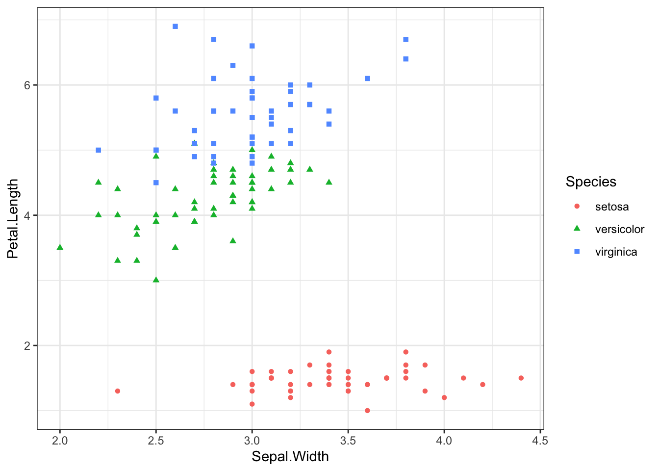

scatter <- ggplot(data=iris, aes(x = Sepal.Length, y = Petal.Width)) 
scatter + geom_point(aes(color=Species, shape=Species))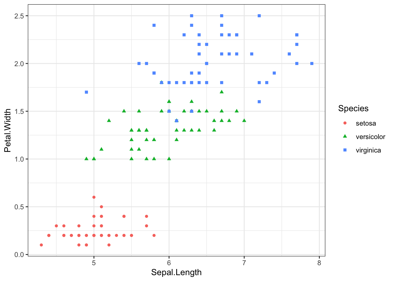

2.3 Prediction target

Say we want to predict the red point with a Petal.With value of 0.6. But assume that this had one error in the recordings, as follows.

## We will predict nr 44
iris[44, , drop=F]

##    Sepal.Length Sepal.Width Petal.Length Petal.Width Species
## 44            5         3.5          1.6         0.6  setosa

## Make prediction hard by introducing an error
iris$Petal.Width[44] = 1.5
## We will predict nr 44
iris[44, , drop=F]

##    Sepal.Length Sepal.Width Petal.Length Petal.Width Species
## 44            5         3.5          1.6         1.5  setosa

This erroneous value is still well within the values in the dataset, and would usually not be removed during data cleaning.

## Prediction target
prediction.cov = iris[44, -5, drop=F]
print(prediction.cov)

##    Sepal.Length Sepal.Width Petal.Length Petal.Width
## 44            5         3.5          1.6         1.5

## Training data
training.cov = iris[-44, -5]
training.class = iris$Species[-44]

3 Models

3.1 Random forest

## See: https://rpubs.com/Jay2548/519589
fit.rf = randomForest(Species ~., data = iris[-44, ],
                  importance = T)
predict(fit.rf, newdata = prediction.cov)

##     44 
## setosa 
## Levels: setosa versicolor virginica

3.2 Naive Bayes

library(e1071)
## We get the wrong prediction
fit.nb=naiveBayes(Species~., iris[-44, ])
pred.nb.1=predict(fit.nb, prediction.cov)
pred.nb.1

## [1] versicolor
## Levels: setosa versicolor virginica

## But if we set the broken data to NA it works:
temp = prediction.cov
temp$Petal.Width = NA
pred.nb.2=predict(fit.nb, temp)

## Warning in predict.naiveBayes(fit.nb, temp): Type mismatch between
## training and new data for variable 'Petal.Width'. Did you use factors
## with numeric labels for training, and numeric values for new data?

pred.nb.2

## [1] setosa
## Levels: setosa versicolor virginica

3.3 NBP

## Fit and predict:
nbp = NBP_classify(training.cov, training.class, prediction.cov)
nbp

##      row_names  nbp_class    covariate   p_val  logdens
## 1           44     setosa Sepal.Length 1.0e+00   0.1135
## 1.1         44     setosa  Sepal.Width 7.9e-01   0.0071
## 1.2         44     setosa Petal.Length 5.7e-01   0.6634
## 1.3         44     setosa  Petal.Width 0.0e+00 -95.9687
## 11          44 versicolor Sepal.Length 8.1e-02  -1.7777
## 1.11        44 versicolor  Sepal.Width 2.6e-02  -2.2480
## 1.21        44 versicolor Petal.Length 4.9e-09 -17.2877
## 1.31        44 versicolor  Petal.Width 3.1e-01   0.1904
## 12          44  virginica Sepal.Length 1.8e-02  -3.2485
## 1.12        44  virginica  Sepal.Width 1.2e-01  -0.9892
## 1.22        44  virginica Petal.Length 8.2e-13 -25.9370
## 1.32        44  virginica  Petal.Width 6.9e-02  -1.2838

Aggregate prediction

pagg = NBP_aggregate_p_values(nbp$p_val, by=nbp[, c("row_names","nbp_class"), drop=F])
pagg

##   row_names  nbp_class   p_val
## 1        44     setosa 7.3e-03
## 2        44 versicolor 4.0e-05
## 3        44  virginica 1.2e-05

pagg$nbp_class[which.max(pagg$p_val)]

## [1] "setosa"

4 Bonus material

4.1 Computing W

W is the discrete point prediction vector, with a 0 or 1 for each category. If the model does not know which category the prediction belongs to this is represented as several 1’s in this vector.

NBP_pred_categories(pagg)

##   row_names  nbp_class p_val
## 1        44     setosa     1
## 2        44 versicolor     0
## 3        44  virginica     0

4.2 Naive Bayes with NBPclassify

Future update: TODO: Show how to compute NB with the package. To get the same results as the NB code above.

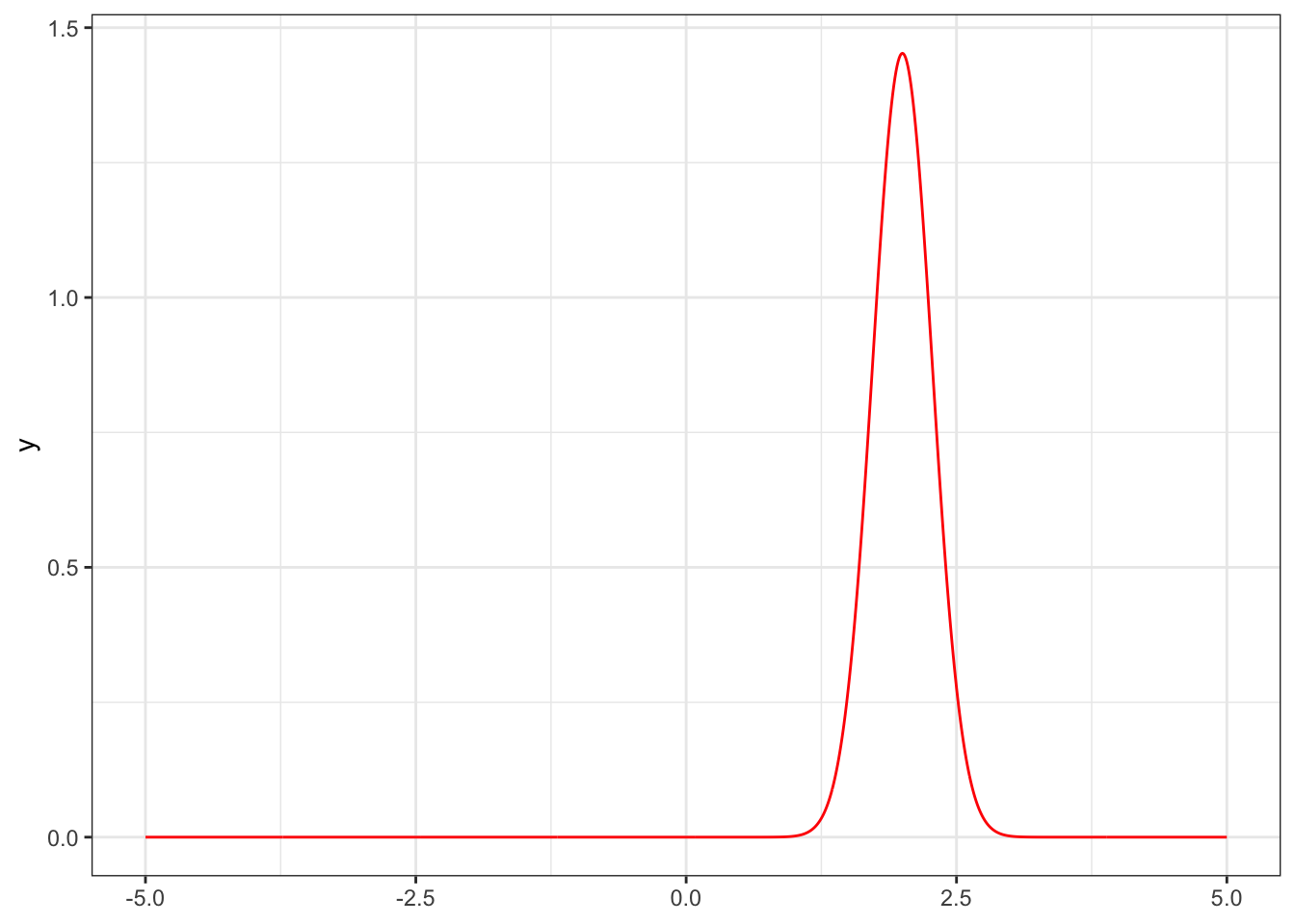
4.3 Density plots

There is a hidden feature of the package that allows you to extract the “Naive Bayes” density functions. This is convenient for plotting.

## Test keep
ptab2 = NBP_classify(training.cov, training.class, prediction.cov, keep = T)

flist = attr(ptab2, "flist")

fun1 = flist[[1]][[1]]

ggplot() + xlim(-5, 5) + theme_bw()  +
  geom_function(fun = fun1, colour = "red", n=1001)

How to use the NBPclassify package on the iris data

Haakon Bakka

Btopic 136 updated 25 April 2023